Population data help the businessman considerably in exploring new markets for his product; they serve as guideposts to market demand. The information on the consumer’s preference, buying habits, levels of living and income, together with their competition to be met, and the cost of operating business should be carefully studied.
It should be noted that not all commodities enjoy large sales even in communities that are thickly populated. Hence, a dealer in working clothes should take into account the number of farmers and laborers in the community, not the total population. Dealers in tractors, in farm machineries, and in agricultural implements may use agricultural income as a good index in determining their sales potentials. Dealers in gasoline should consider the number of motor vehicles in the place of business as a good measure of probable volume of sales.
kinds of set
Tuesday, August 31, 2010
The "I'm Pooped" Menu lol..
I feel another bout of Mono coming on..nooooooooooooo lol.
I'm very fatigued and everything hurts, lymph nodes saying mmmhello, all
that good stuff. I have a round of it every fall and spring.
So this is my menu tonight when I cook:
double batch SOS
double batch cream of broccoli soup
Spam pizza
dessert will be egg free cake or one bowl chocolate brownies
two loaves of white bread.
It's lovely, braindead, and to the point lol!
marapets word search answers
M7N1c - Integers
M7N1. Students will understand the meaning of positive and negative rational numbers and use them in computation.
c. Add, subtract, multiply, and divide positive and negative rational numbers.
I usually don't venture into the 6-8 standards. But, since we discussed the compensation strategies recently, I thought I would discuss how two of those strategies can be used to derive the methods of calculations with integers.
Recall that the equal addition principle of subtraction states that if we add (or subtract) the same number to both the minuend and the subtrahend, the difference stays the same. Thus, 93 - 18 = (93 + 2) - (18 + 2) = 95 - 20. Another property of subtraction students encounter early on is that subtracting 0 will not change the number, that is A - 0 = A. By combining these two properties of subtracti! on, we can think about a problem like 8 - (-3) this way:
"We know subtracting 0 does not change the number. So, what can I do to change the subtrahend (-3) to 0? Add 3. But, the equal addition principle of subtraction says I have to add the same number to the minuend to keep the difference the same. So,
8 - (-3) = (8 + 3) - (-3 + 3) = (8 + 3) - 0 = 8 + 3."
Thus, you can see that subtracting a negative number is the same as adding the opposite.
We noted that there is a parallel between the compensation strategies for subtraction and division. We can actually use the equal multiplication principle of division to think about division of fraction problems, by combining it with another parallel property, dividing by 1 does not change the number. So, if you are given 3/5 ÷ 2/3, we can think like this:
"We know dividing by 1 does not change the number. So, how can we change (2/3), the divisor, into 1? Multiply by its reci! procal, of course. But the equal multiplication principle of ! division says I will have to multiply the dividend by the same number, too. So,3/5 ÷ 2/3 = (3/5 x 3/2) ÷ (2/3 x 3/2) = (3/5 x 3/2) ÷ 1 = 3/5 x 3/2."
Thus, we see that the division of fractions is the same as the multiplication by the reciprocal of the divisor.
Of course, strictly speaking, there is a minor glitch in both of these arguments. We established the four compensation strategies with whole numbers. But, we don't know if they still hold if we expand the range of numbers to integers/rational numbers. So, there is a circularity in these arguments. So, I'm not advocating these strategies to establish the computation algorithms, specially since there are other ways where students can meaningfully develop algorithms. However, I think these mathematical relationships are still interesting.
learn integers
I usually don't venture into the 6-8 standards. But, since we discussed the compensation strategies recently, I thought I would discuss how two of those strategies can be used to derive the methods of calculations with integers.
Recall that the equal addition principle of subtraction states that if we add (or subtract) the same number to both the minuend and the subtrahend, the difference stays the same. Thus, 93 - 18 = (93 + 2) - (18 + 2) = 95 - 20. Another property of subtraction students encounter early on is that subtracting 0 will not change the number, that is A - 0 = A. By combining these two properties of subtracti! on, we can think about a problem like 8 - (-3) this way:
8 - (-3) = (8 + 3) - (-3 + 3) = (8 + 3) - 0 = 8 + 3."
Thus, you can see that subtracting a negative number is the same as adding the opposite.
We noted that there is a parallel between the compensation strategies for subtraction and division. We can actually use the equal multiplication principle of division to think about division of fraction problems, by combining it with another parallel property, dividing by 1 does not change the number. So, if you are given 3/5 ÷ 2/3, we can think like this:
Thus, we see that the division of fractions is the same as the multiplication by the reciprocal of the divisor.
Of course, strictly speaking, there is a minor glitch in both of these arguments. We established the four compensation strategies with whole numbers. But, we don't know if they still hold if we expand the range of numbers to integers/rational numbers. So, there is a circularity in these arguments. So, I'm not advocating these strategies to establish the computation algorithms, specially since there are other ways where students can meaningfully develop algorithms. However, I think these mathematical relationships are still interesting.
learn integers
Kinds of set
1. Finite set – countable
Example: Sets A, B, C, D are finite sets
2. Infinite set – uncountable
Example: Set E is an infinite set
3. Empty or null set – has no element
Example: A = { }
4. Equal set – set A and set B are equal set if the elements of set A is exactly the element of set B.
Example:
A = {set of an even counting number of one digit} = {2,4,6,8}
B = {set of an integral multiples of two having one digit = {2,4,6,8}
5. Equivalent set – two sets are equivalent if there exists a one-to-one correspondence between elements of the two sets.
Example:
A = {1, 2, 3, 4,5} - x coordinate
B = {6, 7, 8, 9, 10} – y coordinate
then &! #8220;A” is equivalent to B. We can construct the relation of set A and set B.
{ (1,6}, (2,7), (3,8), (4,4), (5,10) }
6. Subset – set whose elements are members of the given set A = {1,2,3,4,5,8}, B = {2,4,8}
7. Universal Set – totality of the given set with consideration. The set from which we select elements to form A given set is called universal.
Example:
Set A = {1, 2, 3, 4, 5, 8} is a universal set
Set B = {2, 4, 8} is a subset of set A
8. Disjoint Set – sets that has no common element ; if two sets have no element in common, the sets are called disjoint sets.
kinds of set
The Music Ensemble/Sports Team analogy
I have two sons who are active Little League players - actually only one now, since my older son has aged out of the league. Both are also very active musicians. Sometimes I'll talk with parents who will make comparisons between team sports and music ensemble experiences. I'll often hear a music rehearsal (or class) compared to a sports team practice, an analogy that doesn't hold up for me. I think of it a little differently. Here are some comparisons, with the sports team concept first, followed by the music ensemble concept.
manager/coach=conductor/instructor (easy enough)
player (athlete)=player (musician) (as easy as it gets)
team practice=practicing instrument/music at home (I'll explain some of these more at the end)
regular season game=music ensemble rehearsal/class
playoff game=performance/concert
You may be asking: "W! hy isn't a rehearsal analogous to a practice and a performance analogous to a game?" Well, in most youth sports programs there are many games that lead up to some form of championship series. In most leagues, such a Little League, regular season games are all about equal playing time (as much as is possible) and learning the game. Team records in Little League are cleared at the beginning of the playoffs - all teams begin the post-season on equal footing. Only in the playoffs do wins and losses determine rank in the league.
In a music ensemble, there tend to be far fewer performances than games in a sports season. In fact, in most American educational ensembles (not just PMAC, but public schools and other music opportunities) there tends to be only one or two performanc! es at the end of a long series of rehearsals. The same weight ! is put o n such performances as is put on sports playoff games. Performances, like playoff games, are taken very seriously, even though the point (like in sports) is to experience the thrill and joy of participation in such an event. Good Little League programs are able to balance fun with the gravity of a playoff game, and good music programs are able to balance fun with the gravity of live performance in front of an audience.
Regular season games are very important. Each season I see my sons' teams improve vastly, especially in the area of defense (which is the aspect of baseball that requires the most team interaction), over the course of the regular season. It is the regular season games that provide the educational atmosphere that make compelling and well-played playoff games possible.
A baseball game can't be played without all 9 fielders, and some pitching and fielding relief in the dugout. Basically, a team plays at its best when everyone is present. The! same holds true for music ensembles. Whether an orchestra, rock band or sax quartet, all ensembles play their best when everyone is present. In a music ensemble, the need for all members to be present and playing is analogous to a team's need for all players at a regular season game.
In sports teams, practices are opportunities isolate fundamentals and work on drills. I see this as analogous to practicing one's part at home or in private lessons with a teacher. Just as a sports team can't run onto the field and play a game without practicing drills and learning rules in practice, a music ensemble can't play pieces of music in a rehearsal without the players practicing and learning their parts independently. Just as baseball players will practice fielding ground balls during drills at their team practice, music students should! be prac ticing isolated passages from their music in independent practice sessions and lessons. Yes, the first several rehearsals are spent putting isolated parts of music together, but in most music ensembles entire pieces are being played after the first couple rehearsals (if not from the very first rehearsal). And once the musical group starts playing full pieces in rehearsal, independent practice does not stop, but rather continues to be an important part of the preparation cycle.
As with all analogies, these comparisons are not iron-clad definitions. I present them purely to demonstrate expectation similarities. Similar to sports, each player in a music ensemble plays a specific, unique role. And as such, each player is as indispensable to their ensemble as a player is to his team.
In rehearsals, much like sports games, the absence of players creates challenges that are sometimes impossible! to overcome. When there aren't enough players to field, games are forfeited, and teams miss the opportunity to prepare for the playoffs. When playing in an ensemble, the same level of commitment is expected of a musician as is expected of an athlete on a sports team. And when student musicians rise to the occasion, remarkable things happen. That is why a spectacular music performance can often give audiences the same feelings of excitement and joy that sports fans experience during a playoff win.
is to as is to analogy
A COMSOL Multiphysics Application : Induction Stirred Ladle
Hi All,
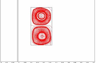
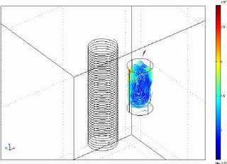
I am posting today a sample Comsol Multiphyiscs application Model. I am Presenting a model in Femlab of induction stirred ladle furnace. The geometry of the model is shown in figure 1. 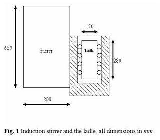
There is a induction coil which produces magnetic field. It is placed near a cylindrical ladle containing a conducting fluid or motlen steal.
The Basic governing equation are the well known Maxwells equation which gives the magnetic field in terms of a Magentic Diffusion equation given as:
dB/dt = 1/(sigma*mu)*(del^2(B)) --------------- (1)
The Solution of the above Magnetic diffusion equation will give the Magnetic field Bx, By and Bz as a function of time. These Magnetic field can then be used to find the Lorenz Force which will induce motion of the Melt/molten liquid inside the ladle. Given as :
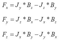 These force field are fed into the NS or K-e model as source term for obtaining the solution of the velocity field in the melt. The Modelling is then done as follows:
I tried to model it in 2 D and 3 D. Although 3 D model is more accurate. W! hile modelling in 2D I assumed that the magnetic filedis in Bx! and By direction only. The interaction of magnetic field and induced current will produce Lorenz force which will rotate the liquid metal in the cylindrical ladle placed near the induction coil. In 3d the inductor is modelled as current carrying coil. The coil geometry is created in MATLAB and then imported into COMSOL. To compute the velocity field in the model, I have coupled the two models using multiphysics option. I have coupled 3D quasi Static and 3D incompressible Navierstokes while modelling in 3D. In 2D modelling I have coupled k-e model and perpendicular current in electomagnetics. Now to solve the problem the the solve manager is used separately. First you solve the Electromagnetics (QAV) problem only, calculating the forces. Then you only solve the Navier Stokes (NS) using these forces. The forces will be constant during this solution process. You do this with the Solver manager under the tab Solve for. Here you select the QAV mode when you solve the qu! asi statics and NS mode for Navier stokes. After the QAVsolution you must select Current solution as initial value. Your Navierstokes problem also need some help in defining the pressure, otherwise it will be undefined. Specify a point constraint in one point under pointsettings to a certain pressure. Also believe that you need denser mesh inthe container where you solve the NS problem.
On running the solver now I do get the solution of the magnetic field and also the induced currents and the melt velocity field. The model here is described in very brief, if any one required more information about current density setting and how to make a coil in MATLAB and how to import in into COMSOL just write a querry on the blog.
The Figure below shows the model in COMSOL in 2 and 3D.
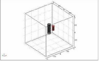
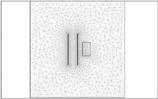
The Results are shown here in 2D and 3D
initial value problem calculator
Vedic Mathematics Lesson 43: Polynomial Division 1
You can find all my previous posts about Vedic Mathematics below:
Introduction to Vedic Mathematics
A Spectacular Illustration of Vedic Mathematics
10's Complements
Multiplication Part 1
Multiplication Part 2
Multiplication Part 3
Multiplication Part 4
Multiplication Part 5
Multiplication Special Case 1
Multiplication Special Case 2
Multipli! cation S pecial Case 3
Vertically And Crosswise I
Vertically And Crosswise II
Squaring, Cubing, Etc.
Subtraction
Division By The Nikhilam Method I
Division By The Nikhilam Method II
Division By The Nikhilam Method III
Division By The Paravartya Method
Digital Roots
Straight Division I
Straight Division II
Vinculums
Divisibility Rules
Simple Osculation
Multiplex Osculation
Solving Equations 1
Solving Equations 2
Solving Equations 3
Solving Equations 4
Mergers 1
Mergers 2
Mergers 3
Multiple Mergers
Complex Mergers
Simultaneous Equations 1
Simultaneous Equations 2
Quadratic Equations 1
Quadratic Equations 2
Quadratic Equations 3
Quadratic Equations 4
Cubic Equations
Quartic Equations
In the previous lesson, we identified one of the solutions to a quartic equation based on the values of the coefficients of the different powers of the unknown variable, x. Once the solution is identified, we needed to perform a polynomial division to get the residual cubic equation from the given quartic equation and one of its solutions. We touched upon the procedure for performing this tangentially, but we did not take it up formally. In this lesson, we will formalize the procedure for performing simple polynomial divisions. In particular, we will deal with the div! ision of higher-order polynomials by polynomials of the first degree (linear polynomials) in this lesson. In future lessons, we will deal with divisions where the divisor is a polynomial of higher degree.
In the most general terms, in this lesson, we are dealing with divisions of the following form:
Divide ax^n + bx^(n-1) + ... + constant by (cx + d)
In the previous lesson, (cx + d) was either (x + 1) or (x - 1). But the method we used in that lesson is applicable to other divisors also. We already know how to do some basic divisions without even realizing we are doing polynomial division. As in any other division, the answer will have a quotient and a remainder. In some cases, the remainder may be zero. In some cases, the quotient may be zero too.
Consider the following example of division by a linear polynomial, wh! ich practically anyone can actually perform without any hesita! tion:
Divide 4x^2 + 6x + 7 by 2x.
In this case, c = 2 and d = 0. Just by inspection, we can say that the quotient of this division is 2x + 3, and the remainder is 7. The way to verify whether we obtained the correct answer, just as in the case of arithmetic division is to check whether dividend = quotient * divisor + remainder.
In the above case, we can indeed verify that 4x^2 + 6x + 7 = 2x*(2x + 3) + 7. Thus, we can be confident that our division was correct.
Now, consider another example of polynomial division which may not be readily apparent as polynomial division. Divide 4x^2 + 6x + 7 by 2. In this case c = 0 and d = 2. Once again, just be inspection, we can say that the quotient is 2x^2 + 3x + 3, and the remainder is 1. We can verify that this is the correct answer by seeing that 4x^2 + 6x + 7 = 2*(2x^2 + 3x + 3) + 1.
However, when neither c nor d is zero, the situation becomes trickier. That is the kind of divisio! n that is not dealt with in school in any detail. It is the kind of division that is not taught to students as a normal part of algebra education for whatever reason. It is actually very useful to teach this kind of division, as we will see later in this lesson!
Consider the division of 4x^2 + 6x + 7 by x + 2. Essentially, we have to find (4x^2 + 6x + 7)/(x + 2). How exactly do we perform this division? The answer turns out to be quite simple actually. We have already seen some examples of how we do such a division in the previous lesson. Let us formalize the method in this lesson.
Consider the division of a polynomial ax^n + bx^(n-1) + ... + constant by the first degree expression cx + d. Consider the ratio c/d. The secret to polynomial division is to rewrite the numerator using this ratio just like we did in our lessons on cubic equations and quartic equations.
We have to rewrite the dividend in the form below:
ax^n + e! x^(n-1) + fx^(n-1) + ... + yx + zx + constant1 + constant2
And the coefficients have to satisfy the conditions below:
c/d = a/e = f/g = ... = z/constant1
e + f = b
...
y + z = coefficient of x in the given dividend
constant1 + constant2 = constant
In some cases, constant2 could be zero. When that is the case, the division does not have a remainder. When constant2 is not zero, that is the remainder (at least an intermediate remainder) of the division.
Let us see how these rules are applied in the case of (4x^2 + 6x + 7)/(x + 2). In this case, c/d = 1/2. Thus, we have to rewrite the dividend using the ration 1/2.
4x^2 + 6x + 7 = 4x^2 + ax + bx + constant1 + constant2
where
1/2 = 4/a = b/constant1
a + b = 6
constant1 + constant2 = 7
We see that we can accomplish this by writing the dividend as below:
4x^2 + 8x - 2x - 4 + 11
This can then be factorized as below:
4x(x + 2) - 2(x + 2) + 11
Consider (4x^3 + 6x^2 - 8x + 15)/(2x - 1). In this case, c/d = -2/1. Thus, we rewrite the dividend using this ratio as below:
4x^3 -2x^2 + 8x^2 - 4x - 4x + 2 + 13
We can then factorize the expression above as below:
2x^2(2x - 1) + 4x(2x - 1) - 2(2x - 1) + 13
Thus, the quotient of the division is 2x^2 + 4x - 2, and the remainder is 13.
Now, consider (3x^4 + 4x^3 - 11x^2 + 6x - 5)/(2x + 1). In this case c/d = 2/1. Thus, we rewrite the dividend using this ratio as below:
3x^4 + 1.5x^3 + 2.5x^3 + ! 1.25x^2 - 12.25x^2 - 6.125x + 12.125x + 6.0625 - 11.0625
!
We can then factorize the expression as below:
1.5x^3(2x + 1) + 1.25x^2(2x + 1) - 6.125x(2x + 1) + 6.0625(2x + 1) - 11.0625
The quotient is then (1.5x^3 + 1.25x^2 - 6.125x + 6.0625), and the remainder is -11.0625. We can rewrite the quotient as 24x^3/16 + 20x^2/16 - 98x/16 + 97/16, and the remainder as -177/16. Thus, the quotient can be rewritten as (24x^3 + 20x^2 - 98x + 97)/16, and the remainder is -177/16.
Thus, we see that the quotient and remainder can contain fractional terms. And, in this case, the remainder was negative too! Thus, polynomial division can result in some results that can cause us to scratch our heads. But, we can verify that the answer we got is correct by simply multiplying the quotient with the divisor, and adding the remainder to the result to see whether we get back our original dividend.
Now consider a division as below:
(2x^3 + 5x^2 - 6x + 8)/(2x + 2)
We see that the ratio c/d ! in this case is 2/2 = 1. Thus, we could rewrite the dividend expression as below:
2x^3 + 2x^2 + 3x^2 + 3x - 9x - 9 + 17
We would then factorize it as below:
2x^2(x + 1) + 3x(x + 1) - 9(x + 1) + 17
We immediately see that the expressions in the parentheses are x + 1, not our divisor, 2x + 2. Thus, if we decide, based on the factorization, that our quotient is 2x^2 + 3x - 9, with a remainder of 17, we will find that we are wrong. In fact, (2x^2 + 3x - 9)(2x + 2) + 17 = 4x^3 + 10x^2 - 12x - 1, which is not what we started with as our original dividend. This, then tells us that the actual factorization of the rewritten dividend is as below:
x^2(2x + 2) + (3x/2)(2x + 2) - (9/2)(2x + 2) + 17
Thus, the quotient would be (x^2 + 3x/2 - 9/2) and the remainder would be 17. This can be verified as the correct answer. Thus, we need to pay extra attention when the ratio c/d can be simplified by the presence of common! factors. The common factor, in this case, prevented us from ! getting the divisor as a common factor during the factorization when we factorized the rewritten dividend. We then had to introduce fractions during the factorization to get the divisor as the common factor during the factorization.
A simpler solution to the above problem would be to take the common factor out of the divisor and divide the dividend by this common factor in advance. In this case, the common factor in the divisor is 2. So, we can convert the dividend to x^3 + (5/2)x^2 - 3x + 4 before we attempt the division. Now, our division problem is reduced to (x^3 + (5/2)x^2 - 3x + 4)/(x + 1). The ratio of terms in the divisor is 1/1 = 1. Thus, we can perform the division by rewriting the dividend as below:
x^3 + x^2 + (3/2)x^2 + (3/2)x - (9/2)x - 9/2 + 17/2
This will then enable us to perform the factorization as below:
x^2(x + 1) + (3x/2)(x + 1) - (9/2)(x + 1) + 17/2
The quotient is then x^2 + 3x/2 + 9/2. But since w! e divided the numerator and denominator by the common factor, 2, remember that the remainder is now to be multiplied by this common factor to get the final remainder. Thus, the remainder is not 17/2, but is instead 17!
Having fractional terms as part of the dividend may appear a little intimidating. So, another solution would be to take the common factor out of the divisor and keep it aside. Perform the division as usual, then divide the resulting quotient by the common factor.
In this case, our initial division resulted in a quotient of 2x^2 + 3x - 9. We see that we can then divide this by the common factor, 2, to get the correct quotient. Remember not to divide the remainder by the common factor!
Now, let us consider the last special case. Consider the division of 6x + 7 by x + 1. In this case, the dividend is also a linear polynomial. But the method is still the same as before. The ratio, c/d, in this case is 1/1 = 1. Thus, we r! ewrite the dividend expression as below in preparation for fac! torizati on:
6x + 6 + 1
This then leads to the factorization as below:
6(x + 1) + 1
We then conclude that the quotient is 6 and the remainder is 1.
Let us now record our observations about polynomial division, with a first-degree polynomial as the divisor, below:
- The quotient will be a polynomial of one degree lower than the original dividend (thus, if the dividend is also a linear expression, as in our last example, then the quotient will be just a constant with no x term)
- The remainder will be a constant, but can be either positive or negative
- If the divisor has a constant as a common factor, we can set the constant aside, divide by the divisor reduced to lowest terms, then divide the quotient by the common factor to get the correct quotient (no change needs to be made to the remainder)
- Alternatively, we can divide the dividend by the common factor, then perform the division by the div! isor reduced to lowest terms to get the quotient, then multiply the remainder by the common factor to get the correct remainder
As you can see, the division of a polynomial by a linear polynomial is quite easy once the method of ratios is laid out. This is an application of the Madhyamadhyena Adhyamanthyena sutra. Now, as promised, let us examine why this technique is useful. The secret to its usefulness lies in the insight that practically every real number is a polynomial. Consider the number 324, for instance.
324 = 3*10^2 + 2*10 + 4
This is the same as 3x^2 + 2x + 4, where x = 10! In fact, we can even express it is 3x^2 + 3x - 6, where x = 10. In fact there are several ways to express a given number as a polynomial, even using just x = 10. Using a different value of x enables us to rewrite the number in other bases (such as octal, where x = 8, hexadecimal, where x = 16 and binary, where x = 2). Because of this, it is easy to ! see that we can use our insights from polynomial division to p! erform r egular arithmetic division with just as much ease! In fact, this is the practical application of polynomial division that I have been hinting at since the beginning of this lesson!!
Take the case of 324/11 for instance. This can be rewritten as (3x^2 + 2x + 4)/(x + 1), where x = 10. We already know how to do this with no problems. We rewrite the dividend expression as below:
3x^2 + 3x - x - 1 + 5
We then factorize it to get:
3x(x + 1) -1(x + 1) + 5
We then conclude that the quotient is 3x - 1 and the remainder is 5. 3x - 1 when x = 10 is 29. Thus, we have just performed the division, 324/11 and found that the quotient is 29 with a remainder of 5. I encourage you to verify that this is indeed correct! Let us now take on a few more examples to see just how easy the method is.
Take 372/12 for instance. This can be rewritten as (3x^2 + 7x + 2)/(x + 2) where x = 10. The ratio, c/d, is then 1/2. We can th! en rewrite the dividend expression as below, and factorize it:
3x^2 + 6x + x + 2, which can be factorized as
3x(x + 2) + 1(x + 2)
Thus, we see that the quotient is 3x + 1 (or 31 with 10 as the value of x), and the remainder is 0!
Now, let us take a few slightly trickier cases. Consider 412/12, for instance. This can be rewritten as (4x^2 + x + 2)/(x + 2), where x = 10. The ratio, c/d is once again 1/2. Then, the dividend can be rewritten and factorized as below:
4x^2 + 8x - 7x - 14 + 16 which can be factorized as
4x(x + 2) - 7(x + 2) + 16
This then tells us that the quotient is 4x - 7 (or 33, since x = 10), and the remainder is 16. This can not be correct. We can verify using a calculator that the quotient in this case should be 34 and the remainder should be 4. It turns out that our solution is correct, but it does not meet the standards for normal division. In particular, in this case, the remainder ! turned out to be bigger than the divisor. To correct this, ad! d one to the quotient and reduce the remainder by the divisor. If necessary, repeat the operation until the remainder becomes less than the divisor. Following this procedure, we can then adjust our solution to a quotient of 34 (add one to 33), and a remainder of 4 (subtract the divisor, 12, from the original remainder of 16). Now, we can say that the answer is in truly correct form!
Now consider the case of 271/13. This can be rewritten as (2x^2 + 7x + 1)/(x + 3), where x = 10. The ratio, c/d is 1/3 in this case. We can then rewrite the dividend expression, and do the factorization as below:
2x^2 + 6x + x + 3 - 2 which can be factorized as
2x(x + 3) + 1(x + 3) - 2
We can then interpret this as saying that the quotient is (2x + 1), or 21 since x = 10, and the remainder is -2. Once again, we are left with an answer that seems wrong. We are not used to dealing with negative remainders when we do divisions normally. But the correction for t! his problem, once again, is very simple. We simply subtract one from the quotient and add the divisor to the remainder. Repeat this until the remainder is positive. Thus, we can correct our answer to a quotient of 20 (subtract 1 from 21), and a remainder of 11 (add the divisor, 13, to -2). It is easy to verify that a quotient of 20 and a remainder of 11 is indeed correct.
Next, let us consider 4878/18. We can write it as (4x^3 + 8x^2 + 7x + 8)/(x + 8), where x = 10. But the ratio, c/d now becomes 1/8. Using that ratio, we would be forced to rewrite the dividend expression as below:
4x^3 + 32x^2 - 24x^2 - 192x + 199x + 1592 - 1584
Obviously, this is correct, and does give us the following factorization:
4x^2(x + 8) - 24x(x + 8) + 199(x + 8) - 1584
This then translates to a quotient of 4x^2 - 24x + 199, which equals 400 - 240 + 199 = 359, and a remainder of -1584. To get this answer to standard form would require ! a lot of subtractions of 1 from the quotient and additions of ! 18 to th e remainder!
Instead, let us consider a different approach to this problem. We can rewrite the given problems as (4x^3 + 8x^2 + 7x + 8)/(2x - 2), where x = 10. Now, we see that c/d = -1 and the divisor has a common factor of 2. Let us take the common factor out initially and do the rewriting and factorization as below:
4x^3 - 4x^2 + 12x^2 - 12x + 19x - 19 + 27 which can be factorized as
4x^2(x - 1) + 12x(x - 1) + 19(x - 1) + 27
This translates to a quotient of 4x^2 + 12x + 19, which can be translated as 539 by substituting x = 10. Now, remember to divide the quotient by 2 (the common factor in the divisor), and we get 269.50. Since the remainder is greater than 18, we also have to subtract 18 from it and add 1 to the quotient. This gives us a quotient of 270.50 and a remainder of 9. Since 0.50*18 is 9, we can further simplify it to a quotient of 270 with a remainder of 18 (subtract the 0.50 from the quotient and add 0.50*18 to the! remainder), which once again can be reduced to a quotient of 271 with no remainder. We can verify that this is indeed the correct answer.
The approach we took the second time around is reminiscent of the use of vinculums in various arithmetic operations. Vinculums are dealt with in great detail in a lesson dedicated to them. It may be useful to review that lesson once more for more insights into the usefulness of the concept of vinculums.
Now, let us consider a more tricky case. We will try 3421/77. This can be rewritten as (3x^3 + 4x^2 + 2x + 1)/(7x + 7), where x = 10. We see that there is a common factor of 7 in the divisor, and a c/d ratio of 1. Using the ratio, we can rewrite the dividend and factorize it as below:
3x^3 + 3x^2 + x^2 + x + x + 1, which can be factorized as
3x^2(x + 1) + x(x + 1) + 1(x + 1)
This directly translates to a quotient of 311 with a remaind! er of 0. We now have to remember to divide the quotient by the common factor, 7. This presents us problems since we are left with another division problem almost as difficult as the original problem. However, we have reduced the problem by at least an order of magnitude, and in fact, we can perform the division by 7 in our heads to get a final quotient of 44 and a remainder of 3. Notice that this remainder is from a division by 7 while the real remainder needs to be from a division by 77. So, to get the true remainder to the problem, we now multiply this remainder of 3 from this step by 77/7 (original divisor/common factor), which is 11. Thus, the final answer is 44 with a remainder of 33.
An easier way to remember this might be to express the answer as 44 and 3/7 with a remainder of 0. Now, we convert the 3/7 to the final remainder by multiplying by the divisor, 77, to get 33 as the final remainder. We can verify that 44*77 + 33 = 8843, so we know our answer is c! orrect.
To obviate the need for a manual division, we can once again the use the concept of vinculums to rewrite the given problem as (3x^3 + 4x^2 + 2x + 1)/(8x - 3). This then gives us a c/d ratio of -8/3. But this leads to new problems as we see below:
3x^3 + 4x^2 + 2x + 1 can be rewritten with a ratio of -8/3 as
3x^3 - (9/8) x^2 + (41/8)x^2 - (123/64)x + (251/64)x - 753/512 + 1264/512 which can be factorized as
(3/8)x^2(8x - 3) + (64/41)x(8x - 3) + (512/251)(8x - 3) + 1264/512
This then gives us a quotient of 300/8 + 640/41 + 512/251 (after substituting x = 10 in the expression above) with a remainder of 1264/512. As you can see, this is not a very convenient expression to work with and convert into a standard form for presentation as a normal quotient and remainder. So, the lesson to take away from this is to be careful and not carried away by vinculums too much!
The concept of polynomial division is useful to le! arn since it can translate directly into an easy method for ar! ithmetic division also. But, sometimes, it does not produce results any faster or easier than other methods of division. This is important to recognize as a shortcoming of the method. Different methods have their own strengths and weaknesses. If the ratio we need to work with is inconvenient and can not be converted into a more convenient ratio by the use of vinculums or other tricks, we have to recognize that polynomial division may not be the best approach to the division problem.
Moreover, in this lesson, we have dealt with only linear divisors. This can limit the technique to just 2-digit divisors under most conditions. We will leave this lesson with an example of a division by a 3-digit divisor, but in general, we will deal with division by more digits in the next lesson, when we will deal with polynomial division where the divisor is not linear.
Consider the division problem 8843/126. This can be expressed as (8x^3 + 8x^2 + 4x + 3)/(x^2 + 2x + 6), ! where x = 10, but this does not leave us with a linear divisor. Instead, let us rewrite this as (8x^3 + 8x^2 + 4x + 3)/(12x + 6), where x = 10. Now, we have a linear divisor, so we can proceed as before. We see that the ratio c/d = 2, and 6 is a common factor in the divisor. We will set aside the common factor for now, and rewrite and factorize the dividend as below:
8x^3 + 4x^2 + 4x^2 + 2x + 2x + 1 + 2 which can be factorized as
4x^2(2x + 1) + 2x(2x + 1) + 1(2x + 1) + 2
This then translates to a quotient of 421, and a remainder of 2. Since we took out a common factor of 6 from the divisor, we now divide the quotient by 6. Dividing 421 by 6 gives us the new quotient of 70 and a remainder of 1. To convert this remainder to a remainder that would be obtained by division by 126 rather than by 6, we need to multiply it by 126/6, which is 21. Now, we add this remainder to the remainder from the factorization to get a final remainder of 23.
An easier way to remember this might be to express the ! result o f the division as 70 and 1/6. To move the 1/6 to the remainder, we need to multiply it by the divisor, 126. This gives us 21, which is then added to the already existing remainder of 2 to give us a final remainder of 23. We can verify that 70*126 + 23 = 8443, so we know that our answer is correct.
As you can see, polynomial division has several uses, chief among them, the factorization of polynomial expressions. But, as we saw in this lesson, it can also translate into an easier way to do some arithmetic divisions also. Hope you will take the time to practice some of the techniques, both with polynomial expressions as well as with arithmetic expressions, so that you can be confident about their application when it is appropriate. Good luck, and happy computing!
how to do polynomials
Subscribe to:
Posts (Atom)